Evaluating Classification performance

![:scale 10%](./imgs/sklearn_logo.png)

#### DSTA Extra Materials

### Evaluating Classification performance

Extra Slides and codes courtesy of [Andreas C. Müller, NYU](https://github.com/amueller/)

---

### Supervised Binary Classification

__Istance:__

- a collection __X__

- its classification __y__  (assume a classification sys. {0,1} or {-1, +1})

__Solution:__ a classifier function (here called *model*)

__Measure:__ misclassification wrt. __y__

---

### C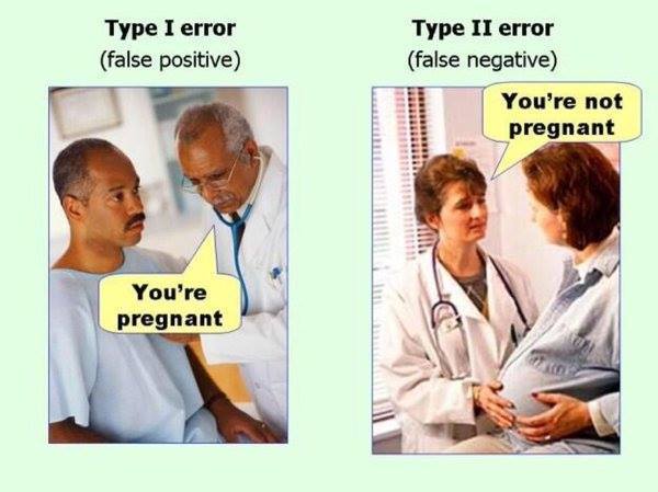onfusion matrix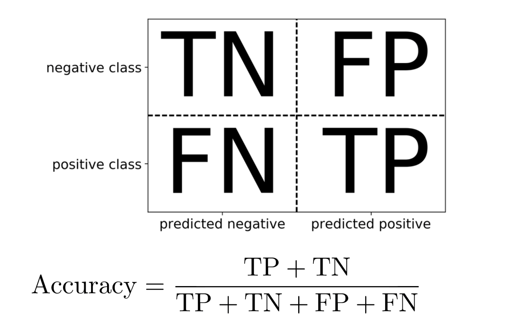

???
Diagonal divided by everything.

---

#### Example: evaluate the *LogisticRegression* classifer

from sklearn.linear_model import LogisticRegression

data = load_breast_cancer()

```
]

---

#### Example: evaluate the *LogisticRegression* classifer

.smaller[
```python
from sklearn.datasets import load_breast_cancer
from sklearn.linear_model import LogisticRegression

data = load_breast_cancer()
```
]

.smaller[
```python
X_train, X_test, y_train, y_test = train_test_split(
    data.data, data.target, stratify=data.target, random_state=0)

lr = LogisticRegression().fit(X_train, y_train)

y_pred = lr.predict(X_test)
```
]

---

#### Example: evaluate the *LogisticRegression* classifer

.smaller[
```python
from sklearn.datasets import load_breast_cancer
from sklearn.linear_model import LogisticRegression
data = load_breast_cancer()

X_train, X_test, y_train, y_test = train_test_split(
    data.data, data.target, stratify=data.target, random_state=0)
lr = LogisticRegression().fit(X_train, y_train)
y_pred = lr.predict(X_test)
```
]

.smaller[
```python
from sklearn.metrics import confusion_matrix
print(confusion_matrix(y_test, y_pred))
print(lr.score(X_test, y_test))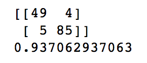
```
]

![:scale 20%](./imgs/breast_cancer_cf_matrix.png)

---

#### Problems with Accuracy

Data with 90% positives:

.smaller[
```python
from sklearn.metrics import accuracy_score
for y_pred in [y_pred_1, y_pred_2, y_pred_3]:
    print(accuracy_score(y_true, y_pred))
```

```
0.9
0.9
0.9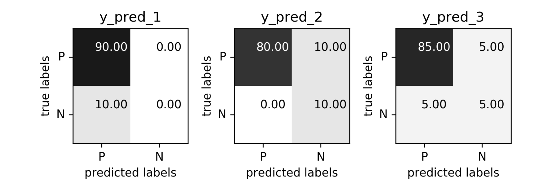
```
]

???
- Imbalanced classes lead to hard-to-interpret accuracy.

---
class:split-40

### Precision, Recall, f-score

.left-column[
`$$ \large\text{Precision} = \frac{\text{TP}}{\text{TP}+\text{FP}}$$` 
`$$\large\text{Recall} = \frac{\text{TP}}{\text{TP}+\text{FN}}$$` 
`$$\large\text{F_1} = 2 \frac{\text{precision} \cdot\text{recall}}{\text{precision}+\text{recall}}$$`]

.right-column[
 
Positive Predicted Value (PPV)
 
 
 
Sensitivity, coverage, true positive rate.
 
 
 
Harmonic mean of precision and recall
]

???
All depend on definition of positive and negative.

---

#### F-score

`$$\large F_1 = 2 \frac{\text{precision} \cdot\text{recall}}{\text{precision}+\text{recall}} = \frac{2}{\frac{1}{\text{precision}}+\frac{1}{\text{recall}}}$$`

Prize on higher recall: `$F_{2}$`

Prize on higher precision: `$F_{0.5}$`

---
class: center, spacious

#### The Zoo

![:scale 100%](./imgs/zoo.png)

https://en.wikipedia.org/wiki/Precision_and_recall

???

---

class:split-40

.right-column[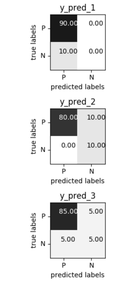
![:scale 20%](./imgs/classification_report_1.png)
 
![:scale 20%](./imgs/classification_report_2.png)
 
![:scale 20%](./imgs/classification_report_3.png)
]

???

---

class:spacious

#### The imporante of experiment design

- What do I want? What do I care about? 
- Can I assign costs to the confusion matrix?
- What guarantees do we want to give?

(the following examples are for `data = load_breast_cancer()`)
???
(precision, recall, or something else)
(i.e. a false positive costs me 10 dollars; a false negative, 100 dollars)

---

#### Setting Thresholds

.tiny-code[
```python
X_train, X_test, y_train, y_test = train_test_split(
    data.data, data.target, stratify=data.target, random_state=0)

lr = LogisticRegression().fit(X_train, y_train)
y_pred = lr.predict(X_test)

print(classification_report(y_test, y_pred))
```
```
          precision   recall  f1-score  support
0              0.91     0.92      0.92       53  
1              0.96     0.94      0.95       90
avg/total      0.94     0.94      0.94      143
```
```python
y_pred = lr.predict_proba(X_test)[:, 1] > .85 # predict 1 only when Pr>.85

print(classification_report(y_test, y_pred))
```
```
          precision   recall  f1-score  support
0              0.84     1.00      0.91       53  
1              1.00     0.89      0.94       90
avg/total      0.94     0.93      0.93      143
```
]

???

---
#### The Precision-Recall curve

SVC: the classifier on the Support Vector Machine algorithm

```python
# [...]

X_train, X_test, y_train, y_test = train_test_split(X, y)

svc = SVC.fit(X_train, y_train)

precision, recall, thresholds = precision_recall_curve(y_test, svc.decision_function(X_test))
```

(some details were omitted)

???
---

#### The Precision-Recall curve of an SVC classifier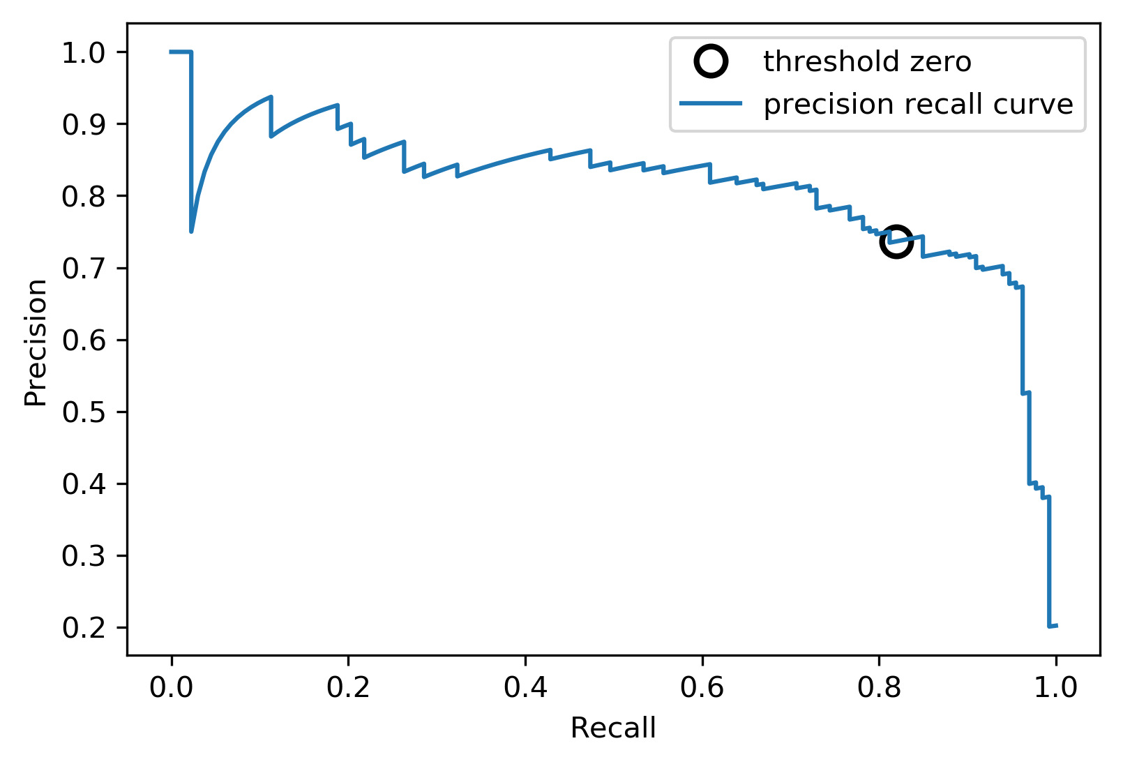

???

---

#### Comparing RF and SVC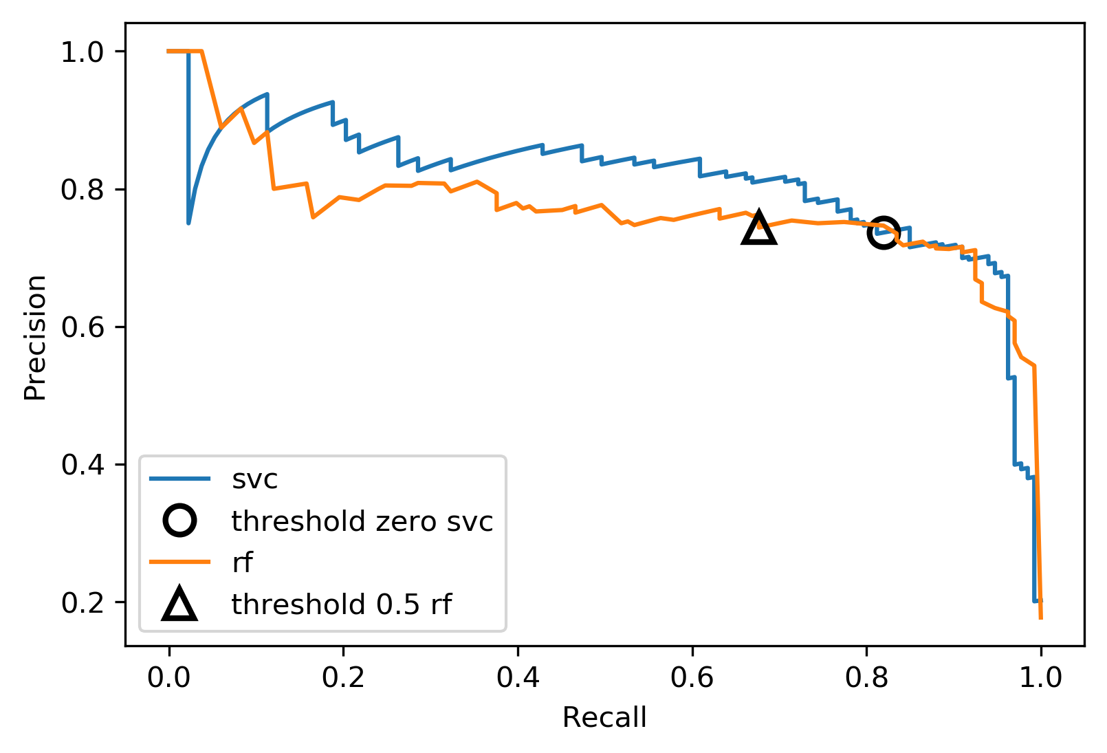

---

#### Alternative: Average Precision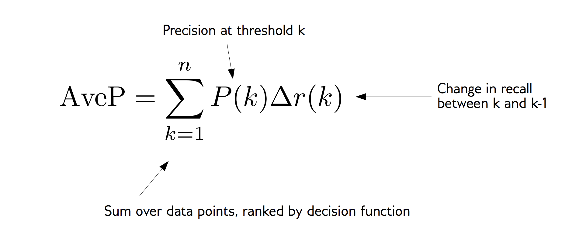

Related to area under the precision-recall curve
(with step interpolation)

---

#### F1 vs. average Precision

print("f1_score of random forest: {:.3f}".format(f1_score(y_test, rf.predict(X_test))))

print("f1_score of svc: {:.3f}".format(f1_score(y_test, svc.predict(X_test))))
```

```
f1_score of random forest: 0.709
f1_score of svc: 0.715
```
```python
from sklearn.metrics import average_precision_score

ap_rf = average_precision_score(y_test, rf.predict_proba(X_test)[:, 1])

ap_svc = average_precision_score(y_test, svc.decision_function(X_test))

print("Average precision of random forest: {:.3f}".format(ap_rf))
print("Average precision of svc: {:.3f}".format(ap_svc))
```
```
Average precision of random forest: 0.682
Average precision of svc: 0.693
```
]
???
AP only considers ranking!
---

#### The ROC Curve

.center[
![:scale 80%](./imgs/zoo.png)
]
`$$ \text{FPR} = \frac{\text{FP}}{\text{FP}+\text{TN}}$$`
`$$ \text{TPR} = \frac{\text{TP}}{\text{TP}+\text{FN}} = \text{recall}$$`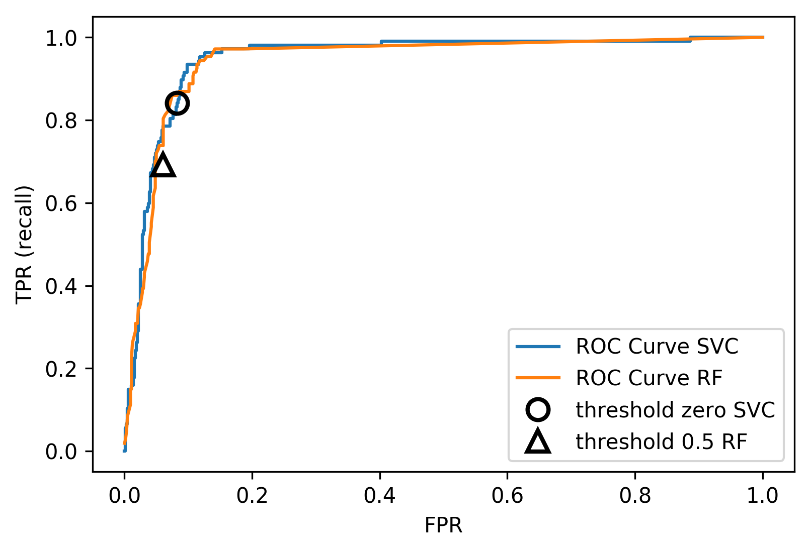
???
---

???
---

#### The ROC AUC

- Area under ROC Curve

- Always .5 for random/constant prediction

rf_auc = roc_auc_score(y_test, rf.predict_proba(X_test)[:,1])

svc_auc = roc_auc_score(y_test, svc.decision_function(X_test))

print("AUC for random forest: {:, .3f}".format(rf_auc))
print("AUC for SVC: {:, .3f}".format(svc_auc))
```

```
AUC for random forest: 0.937
AUC for SVC: 0.916
```
]

Backgorund reading:
*The Relationship Between Precision-Recall and ROC Curves*

https://www.biostat.wisc.edu/~page/rocpr.pdf

???
---

#### Summary of metrics for binary classification

Threshold-based:

- precision, recall,
- accuracy
- `$F_\alpha$`

Ranking-based:

- average precision

- ROC AUC

add log-loss?

???

---

## Non-binary (Multi-class) classification

???

---

class:split-40

#### Confusion Matrix

.left-column[
.tiny-code[
```python
from sklearn.datasets import load_digits
from sklearn.metrics import accuracy_score

digits = load_digits()

# data is between 0 and 16
X_train, X_test, y_train, y_test = 
          train_test_split(digits.data / 16., digits.target, random_state=0)

lr = LogisticRegression().fit(X_train, y_train)

pred = lr.predict(X_test)

print("Accuracy: {:.3f}".format(accuracy_score(y_test, pred)))
print("Confusion matrix:")
print(confusion_matrix(y_test, pred))
```
]
]

---

.tiny-code[
```python
[...]
print("Accuracy: {:.3f}".format(accuracy_score(y_test, pred)))
print("Confusion matrix:")
print(confusion_matrix(y_test, pred))
```

```
Accuracy: 0.964
Confusion matrix:
[[37  0  0  0  0  0  0  0  0  0]
 [ 0 41  0  0  0  0  1  0  1  0]
 [ 0  0 44  0  0  0  0  0  0  0]
 [ 0  0  0 43  0  0  0  0  1  1]
 [ 0  0  0  0 37  0  0  1  0  0]
 [ 0  0  0  0  0 47  0  0  0  1]
 [ 0  1  0  0  0  0 51  0  0  0]
 [ 0  0  0  0  1  0  0 47  0  0]
 [ 0  3  1  0  0  1  0  0 43  0]
 [ 0  0  0  0  0  2  0  0  1 44]]
```
]
]

---

.tiny-code[
```python
print(classification_report(y_test, pred))
```
```
             precision    recall  f1-score   support

0       1.00      1.00      1.00        37
          1       0.91      0.95      0.93        43
          2       0.98      1.00      0.99        44
          3       1.00      0.96      0.98        45
          4       0.97      0.97      0.97        38
          5       0.94      0.98      0.96        48
          6       0.98      0.98      0.98        52
          7       0.98      0.98      0.98        48
          8       0.93      0.90      0.91        48
          9       0.96      0.94      0.95        47

avg / total       0.96      0.96      0.96       450
```
]

???

---

#### Averaging strategies

- "macro", "weighted", "micro" (multi-label), "samples" (multi-label)

`$$\text{macro:  }\frac{1}{\left|L\right|} \sum_{l \in L} R(y_l, \hat{y}_l)$$`

`$$\text{weighted:  } \frac{1}{n} \sum_{l \in L} n_l R(y_l, \hat{y}_l)$$`

print("Macro average: ", recall_score(y_test, pred, average="macro"))
```

```
Micro average: 0.964
Macro average: 0.964
```
]

???
micro vs macro same for other metrics.

---

#### Multi-class ROC AUC

- Hand & Till, 2001, one vs one
`$$ \frac{1}{c(c-1)}\sum_{j=1}^{c}\sum_{k \neq j}^{c} AUC(j,k)$$`

develop a classifier for each pair of possible labels; let them vote on each unseen input

- Provost & Domingo, 2000, one vs rest
`$$ \frac{1}{c}\sum_{j=1}^{c}p(j) AUC(j,\text{rest}_j)$$`

Develop a classifier for each possible label

Apply all of them to an unseen input and that give the label of the corresponding classifier that reports the highest *confidence* score

---

#### observations:

- Accuracy rarely what you want

- Emphasis on recall or precision?

- Problems are rarely balanced

---

#### Available Scikit-learn scoring functions

```python
from sklearn.metrics.scorer import SCORERS

print("\n".join(sorted(SCORERS.keys())))
```
.smaller[
```
accuracy                      log_loss                      precision_micro       
adjusted_mutual_info_score    mean_absolute_error           precision_samples     
adjusted_rand_score           mean_squared_error            precision_weighted   
average_precision             median_absolute_error         r2                   
completeness_score            mutual_info_score             recall               
explained_variance            neg_log_loss                  recall_macro         
f1                            neg_mean_absolute_error       recall_micro         
f1_macro                      neg_mean_squared_error        recall_samples       
f1_micro                      neg_mean_squared_log_error    recall_weighted
f1_samples                    neg_median_absolute_error     roc_auc
f1_weighted                   normalized_mutual_info_score  v_measure_score      
fowlkes_mallows_score         precision                    
homogeneity_score             precision_macro

```
]